Workflow Explanation
How we approach exoplanet analysis and prediction, step by step
Summary
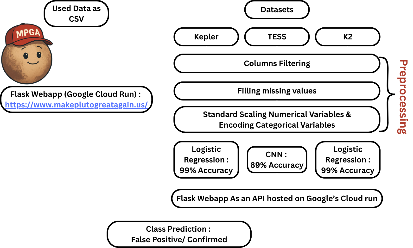
Project Architecture
Project Overview
Our project follows a classic machine learning workflow. We start by collecting data from the Kepler, TESS, and K2 missions. Then, we take a close look at all the features, thinking about what they mean, what values they take, and how useful they might be for making predictions.
Feature Engineering & Data Preprocessing
Removed Features
Limit Features
We took out all features related to "limits" because they were mostly empty or filled with zeros, so they didn't add any value.
Irrelevant Features
We also removed features that didn't help with exoplanet prediction, like IDs or discovery dates, and anything that would make the task too easy or unrealistic.
Example: "sy_pnum" in K2
This feature tells you how many planets have already been found around a star. It doesn't make sense to use it for prediction, because for a new system, we wouldn't know this number in advance. That's exactly what we're trying to figure out!
Preprocessing Pipeline
We built a scikit-learn pipeline to process the data. Here’s what it does:
Columns Filtering
We remove columns that don't help or that would give away the answer.
Filling Missing Values
We fill in missing data using the best method for each column.
Encoding Categorical Variables
We turn text columns into numbers so the model can use them.
Standard Scaling Numerical Variables
We scale the numbers so they're all on a similar range, which helps the model learn.
Kepler Dataset Analysis
Dropped Columns
cols_to_drop = [
    "loc_rowid", "kepid", "kepoi_name", "kepler_name",
    "koi_time0bk", "koi_time0bk_err1", "koi_time0bk_err2",
    "koi_tce_plnt_num", "koi_tce_delivname",
    "ra", "dec",
    "koi_pdisposition",  # Time-series-analysis cheating
    "koi_score"          # Score of cheat
]
All other features were retained for training.
Model Performance
We trained a Logistic Regression model using 5-fold cross-validation and tuned the parameters for best results. Here’s how it performed:
Visualizations
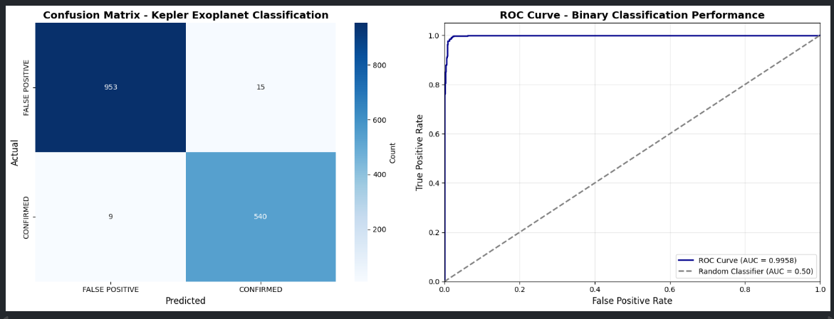
ROC Curve & Confusion Matrix
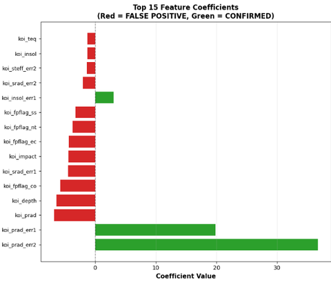
Feature Importance
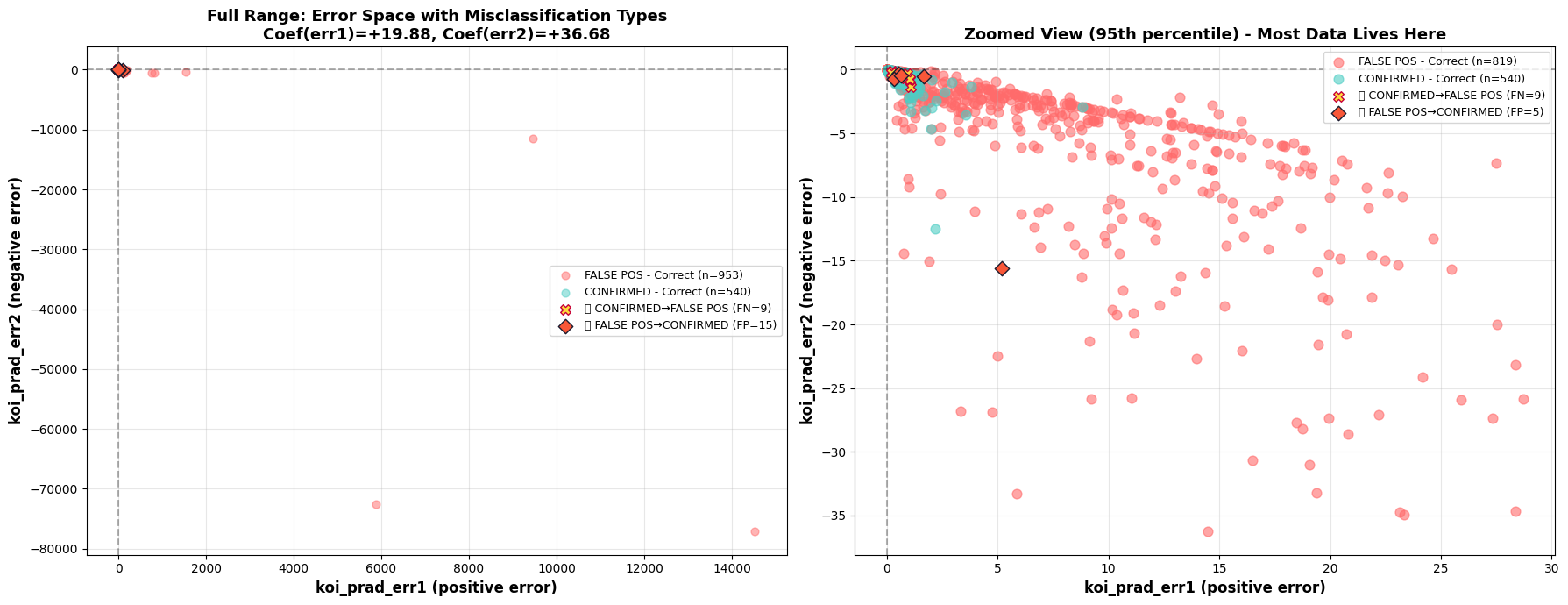
Prediction Visualization on 2 Most Important Features
K2 Dataset Analysis
Used Features
Features: [
    'disposition', 'sy_snum', 'pl_controv_flag', 'pl_orbper',
    'pl_orbpererr1', 'pl_orbpererr2', 'pl_orbsmax', 'pl_orbsmaxerr1',
    'pl_orbsmaxerr2', 'pl_rade', 'pl_radeerr1', 'pl_radeerr2', 'pl_radj',
    'pl_radjerr1', 'pl_radjerr2', 'pl_bmasse', 'pl_bmasseerr1',
    'pl_bmasseerr2', 'pl_bmassj', 'pl_bmassjerr1', 'pl_bmassjerr2',
    'pl_bmassprov', 'pl_orbeccen', 'pl_orbeccenerr1', 'pl_orbeccenerr2',
    'pl_insol', 'pl_insolerr1', 'pl_insolerr2', 'pl_eqt', 'pl_eqterr1',
    'pl_eqterr2', 'ttv_flag', 'st_spectype', 'st_teff', 'st_tefferr1',
    'st_tefferr2', 'st_rad', 'st_raderr1', 'st_raderr2', 'st_mass',
    'st_masserr1', 'st_masserr2', 'st_met', 'st_meterr1', 'st_meterr2',
    'st_metratio', 'st_logg', 'st_loggerr1', 'st_loggerr2', 'sy_dist',
    'sy_disterr1', 'sy_disterr2', 'sy_vmag', 'sy_vmagerr1', 'sy_vmagerr2',
    'sy_kmag', 'sy_kmagerr1', 'sy_kmagerr2', 'sy_gaiamag', 'sy_gaiamagerr1',
    'sy_gaiamagerr2'
]
Target Variable
disposition is the target variable.
Data Filtering Strategy
We left out the candidate rows, since we can't be sure if they're real exoplanets or not. Our goal is to train a model that can tell the difference reliably.
Categorical Encoding
cat_cols_onehot = ["st_spectype", "st_metratio"]
cat_cols_label = ["pl_bmassprov"]
Model Performance
Visualizations
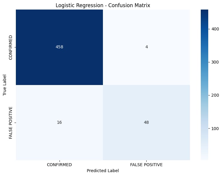
Confusion Matrix
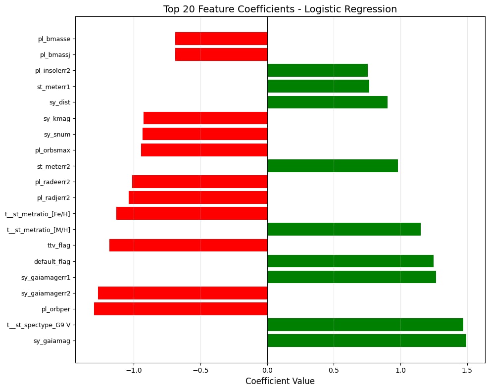
Feature Importance
TESS Dataset Analysis
Most Challenging Dataset
The TESS dataset was the toughest to work with and needed more advanced modeling.
Model Evolution
Phase 1: Traditional ML Models
We started with some classic machine learning models:
- Logistic Regression: 77.7% accuracy
- Decision Tree: 81.16% accuracy
These results were okay, but we wanted to do better.
Phase 2: Autoencoder Architecture
Next, we tried an autoencoder with an extra output for the class prediction.
How it works
The model learns to compress the data into a smaller space, then reconstruct it and predict the class at the same time.
This method gave us an embedding space where the two classes could be separated to some extent:
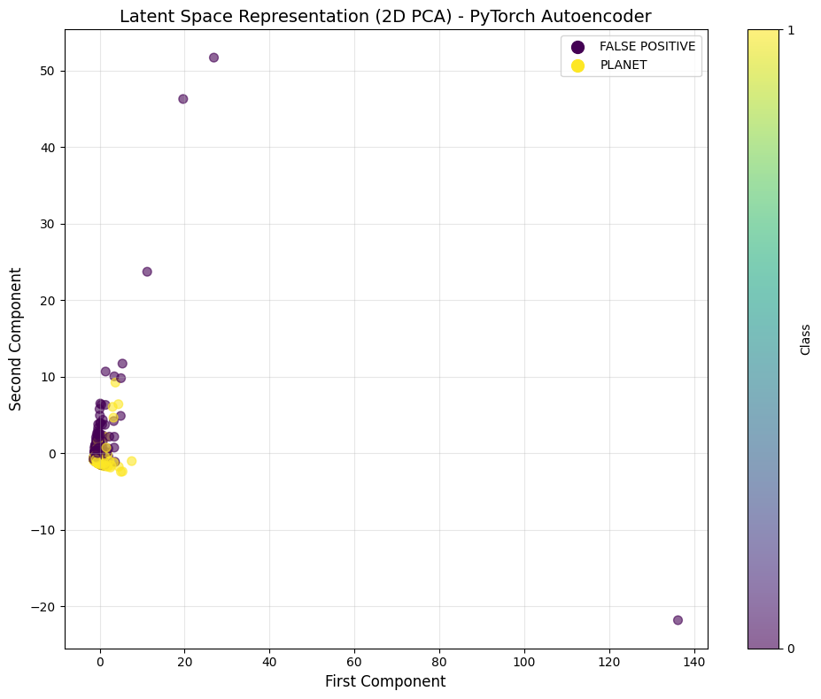
Embedding Space Visualization
Phase 3: 1D Convolutional Neural Network
📚 Inspiration
Inspired by the paper: "Identifying Exoplanets with Deep Learning: A CNN and RNN Classifier for Kepler DR25 and Candidate Vetting"
📄 Read Paper on arXivModel Architecture
1D CNN Model created with 460,929 parameters
Conv1DClassifier(
  (conv_layers): Sequential(
    (0): Conv1d(1, 64, kernel_size=(3,), stride=(1,), padding=(1,))
    (1): BatchNorm1d(64, eps=1e-05, momentum=0.1, affine=True, track_running_stats=True)
    (2): LeakyReLU(negative_slope=0.01)
    (3): Dropout(p=0.2, inplace=False)
    (4): Conv1d(64, 128, kernel_size=(3,), stride=(1,), padding=(1,))
    (5): BatchNorm1d(128, eps=1e-05, momentum=0.1, affine=True, track_running_stats=True)
    (6): LeakyReLU(negative_slope=0.01)
    (7): MaxPool1d(kernel_size=2, stride=2, padding=0, dilation=1, ceil_mode=False)
    (8): Dropout(p=0.2, inplace=False)
    (9): Conv1d(128, 256, kernel_size=(3,), stride=(1,), padding=(1,))
    (10): BatchNorm1d(256, eps=1e-05, momentum=0.1, affine=True, track_running_stats=True)
    (11): LeakyReLU(negative_slope=0.01)
    (12): MaxPool1d(kernel_size=2, stride=2, padding=0, dilation=1, ceil_mode=False)
    (13): Dropout(p=0.2, inplace=False)
  )
  (fc_layers): Sequential(
    (0): Linear(in_features=2560, out_features=128, bias=True)
    (1): BatchNorm1d(128, eps=1e-05, momentum=0.1, affine=True, track_running_stats=True)
    (2): LeakyReLU(negative_slope=0.01)
    (3): Dropout(p=0.2, inplace=False)
    (4): Linear(in_features=128, out_features=64, bias=True)
    (5): BatchNorm1d(64, eps=1e-05, momentum=0.1, affine=True, track_running_stats=True)
    (6): LeakyReLU(negative_slope=0.01)
    (7): Dropout(p=0.2, inplace=False)
    (8): Linear(in_features=64, out_features=1, bias=True)
    (9): Sigmoid()
  )
)📈 Performance Visualizations
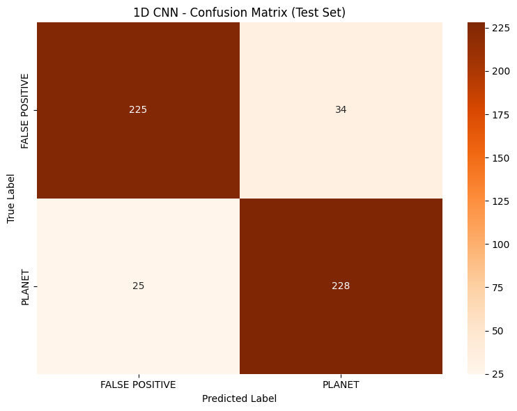
CNN Confusion Matrix
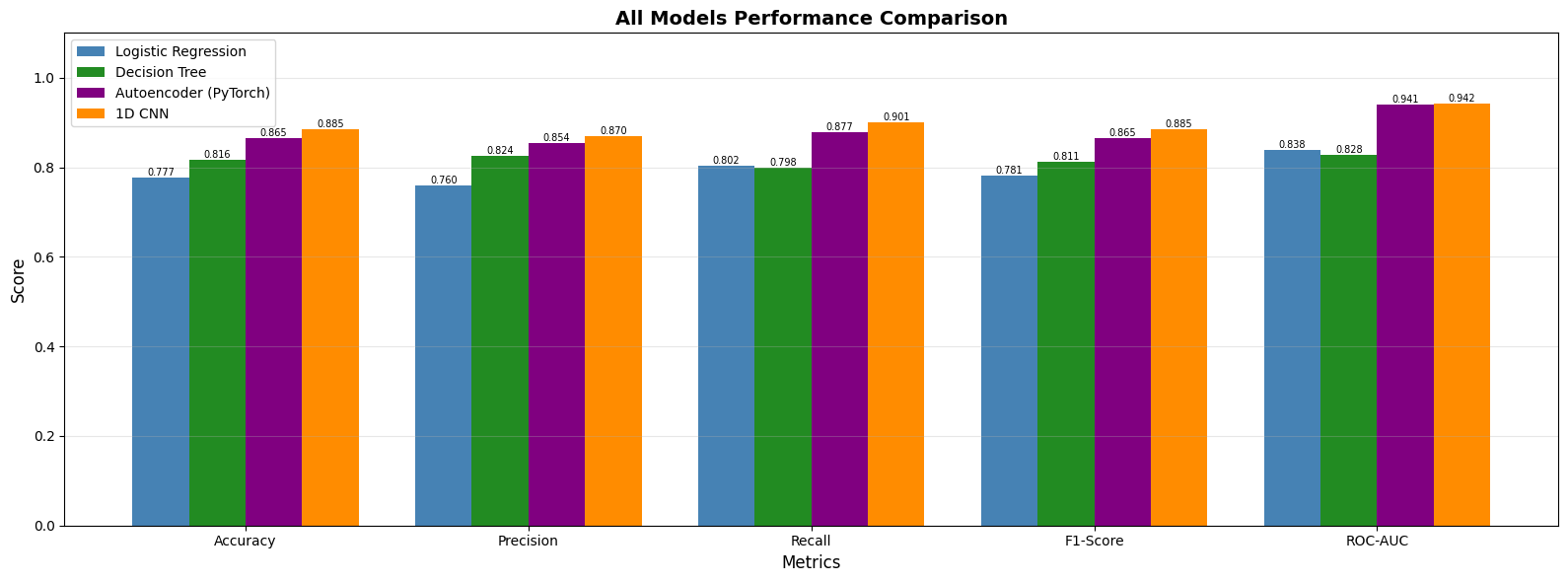
Models Comparison
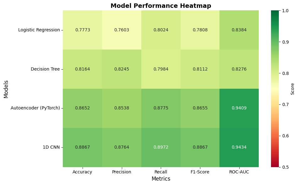
Models Performance Heatmap
Conclusion
Our approach to exoplanet detection is based on careful feature engineering, solid data processing, and trying out different machine learning models until we found what worked best.
Each dataset had its own challenges, so we had to adapt our methods for each one:
- Kepler: 98.42% accuracy with a tuned Logistic Regression model
- K2: 99.13% precision by filtering out uncertain candidates
- TESS: Improved from 77.7% to 88.5% by moving to more complex neural networks